TEBD time evolution

Time-evolving block decimation (TEBD) approximates the propagator by a sequence of local Suzuki–Trotter gates. This example keeps the main comparison visible: evolve a pure-state MPS in Hilbert space, then evolve its vectorized density matrix in Liouville space.

Both representations describe the same closed-system physics. This page keeps a compact Hilbert/Liouville comparison.

Transverse-field Ising model

We study

\[H=-J\sum_{j=1}^{N-1}Z_jZ_{j+1}-h\sum_{j=1}^{N}X_j\]

from the product state $|\psi(0)\rangle=|\mathrm{Up}\cdots\mathrm{Up}\rangle$.

using ITensors
using LinearAlgebra
using ProcessTensors
using ITensors.Ops: Trotter

const N = 4
const J = 1.0
const h = 1.2
const dt = 0.1
const final_time = 2.0
const nsteps = round(Int, final_time / dt)
const maxdim = 64
const cutoff = 1e-12

sites = siteinds("S=1/2", N)
liouville_sites = liouv_sites(sites)

H = let H_local = OpSum()
    for j in 1:(N - 1)
        H_local += -J, "Z", j, "Z", j + 1
    end
    for j in 1:N
        H_local += -h, "X", j
    end
    H_local
end

H_mpo = MPO(H, sites)
initial_state = MPS(sites, fill("Up", N))
initial_density = to_dm(initial_state)
initial_density_liouville =
    to_liouville(initial_density; sites=liouville_sites)

mean_x = let observable = OpSum()
    for j in 1:N
        observable += 1 / N, "X", j
    end
    observable
end
mean_x_mpo = MPO(mean_x, sites)
mean_x_liouville = to_liouville(mean_x_mpo; sites=liouville_sites)

@assert isapprox(real(inner(initial_state, initial_state)), 1; atol=1e-12)

Exact small-system reference

Exact diagonalization is practical here only because $N=4$. The tensor contractions below expose the dense Hamiltonian, initial state, and mean-spin observable directly. These will later be compared to the TEBD results we obtain using our tebd function.

dimension = prod(dim.(sites))

H_tensor = foldl(*, H_mpo)
H_dense = reshape(
    ComplexF64.(Array(H_tensor, prime.(sites)..., sites...)),
    dimension,
    dimension,
)

state_tensor = foldl(*, initial_state)
state_dense = vec(ComplexF64.(Array(state_tensor, sites...)))
density_dense = state_dense * state_dense'

mean_x_tensor = foldl(*, mean_x_mpo)
mean_x_dense = reshape(
    ComplexF64.(Array(mean_x_tensor, prime.(sites)..., sites...)),
    dimension,
    dimension,
)

function exact_density_at(
    time::Real,
    H_dense::AbstractMatrix,
    density0::AbstractMatrix,
)
    propagator = exp(-1im * time * H_dense)
    return propagator * density0 * propagator'
end

function exact_sx_trajectory(
    H_dense::AbstractMatrix,
    density0::AbstractMatrix,
    mean_x_dense::AbstractMatrix,
    times::AbstractVector,
)
    return [
        real(tr(exact_density_at(time, H_dense, density0) * mean_x_dense))
        for time in times
    ]
end

times = collect(range(0.0; step=dt, length=nsteps + 1))
sx_exact =
    exact_sx_trajectory(H_dense, density_dense, mean_x_dense, times)

21-element Vector{Float64}:
 0.0
 0.03496372728313803
 0.12811205978038065
 0.24902343563310836
 0.36082575081470475
 0.4343349976997018
 0.4579367695107651
 0.4392972906550874
 0.39895914353998235
 0.3595560318607647
 0.3360003028941427
 0.33090919812986364
 0.33649597183522306
 0.3408572148680193
 0.3347427021501954
 0.3153140117720465
 0.2856265202140134
 0.2511992141585857
 0.21653764043956134
 0.18405703284433284
 0.1558864344383244

Hilbert-space TEBD

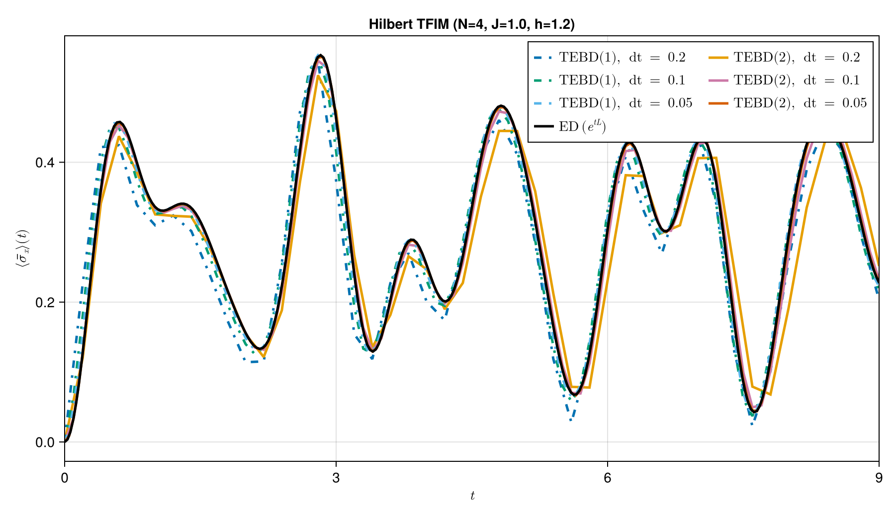
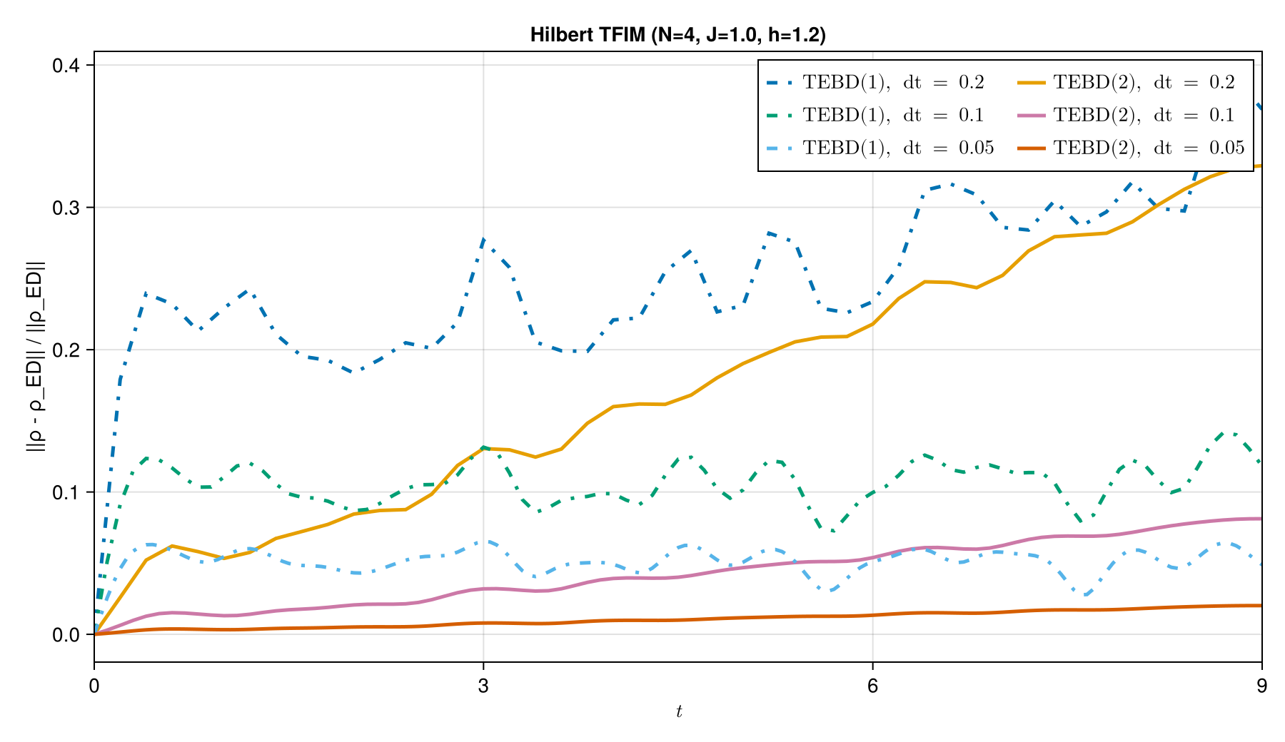
In Hilbert space, tebd applies the Hamiltonian gates directly to $|\psi\rangle$. We use second-order Trotter splitting and record $\langle\bar X\rangle$ after every step.

hilbert_trajectory = let
    state = copy(initial_state)
    sx = Float64[real(inner(state', mean_x_mpo, state))]
    elapsed = 0.0
    for _ in 1:nsteps
        elapsed += @elapsed state = tebd(
            state,
            H,
            dt,
            dt;
            alg=Trotter{2}(),
            maxdim=maxdim,
            cutoff=cutoff,
        )
        push!(sx, real(inner(state', mean_x_mpo, state)))
    end

    (; state, sx, elapsed)
end

hilbert_density = to_dm(hilbert_trajectory.state)
hilbert_density_tensor = foldl(*, hilbert_density)
hilbert_density_dense = reshape(
    ComplexF64.(
        Array(hilbert_density_tensor, prime.(sites)..., sites...)
    ),
    dimension,
    dimension,
)

exact_final_density =
    exact_density_at(final_time, H_dense, density_dense)
hilbert_error =
    norm(hilbert_density_dense - exact_final_density) /
    norm(exact_final_density)

println("TEBD(2) on Hilbert space with dt=$(dt)")
println("    Wall time to final state: $(round(hilbert_trajectory.elapsed, digits=4)) s")
println("    Norm error of the final matrix: $(round(hilbert_error, digits=6))")
println("    Max bond dim of final state: $(maxlinkdim(hilbert_trajectory.state))")

@assert all(isfinite, hilbert_trajectory.sx)
@assert hilbert_error < 0.05

TEBD(2) on Hilbert space with dt=0.1
    Wall time to final state: 0.0908 s
    Norm error of the final matrix: 0.020653
    Max bond dim of final state: 4

The Hilbert-space dynamics and density-matrix error against ED look like:

Liouville-space TEBD

In Liouville space, the state is $|\rho\rangle\rangle$ and the same public tebd function constructs the commutator Liouvillian internally. No jump operators are supplied, so this remains closed unitary dynamics.

empty_jumps = Tuple{Number,String,Int}[]

liouville_trajectory = let
    density = copy(initial_density_liouville)
    sx = Float64[real(inner(mean_x_liouville, density))]
    elapsed = 0.0
    for _ in 1:nsteps
        elapsed += @elapsed density = tebd(
            density,
            H,
            dt,
            dt;
            jump_ops=empty_jumps,
            alg=Trotter{2}(),
            maxdim=maxdim,
            cutoff=cutoff,
        )
        push!(sx, real(inner(mean_x_liouville, density)))
    end

    (; density, sx, elapsed)
end

liouville_density = to_hilbert(liouville_trajectory.density)
liouville_density_tensor = foldl(*, liouville_density)
liouville_density_dense = reshape(
    ComplexF64.(
        Array(liouville_density_tensor, prime.(sites)..., sites...)
    ),
    dimension,
    dimension,
)

liouville_error =
    norm(liouville_density_dense - exact_final_density) /
    norm(exact_final_density)

println("TEBD(2) on Liouville space with dt=$(dt)")
println("    Wall time to final state: $(round(liouville_trajectory.elapsed, digits=4)) s")
println("    Norm error of the final matrix: $(round(liouville_error, digits=6))")
println("    Max bond dim of final state: $(maxlinkdim(liouville_trajectory.density))")

@assert all(isfinite, liouville_trajectory.sx)
@assert maximum(abs.(hilbert_trajectory.sx - sx_exact)) < 0.05
@assert maximum(abs.(liouville_trajectory.sx - sx_exact)) < 0.05
@assert liouville_error < 0.05

TEBD(2) on Liouville space with dt=0.1
    Wall time to final state: 0.2153 s
    Norm error of the final matrix: 0.020653
    Max bond dim of final state: 16

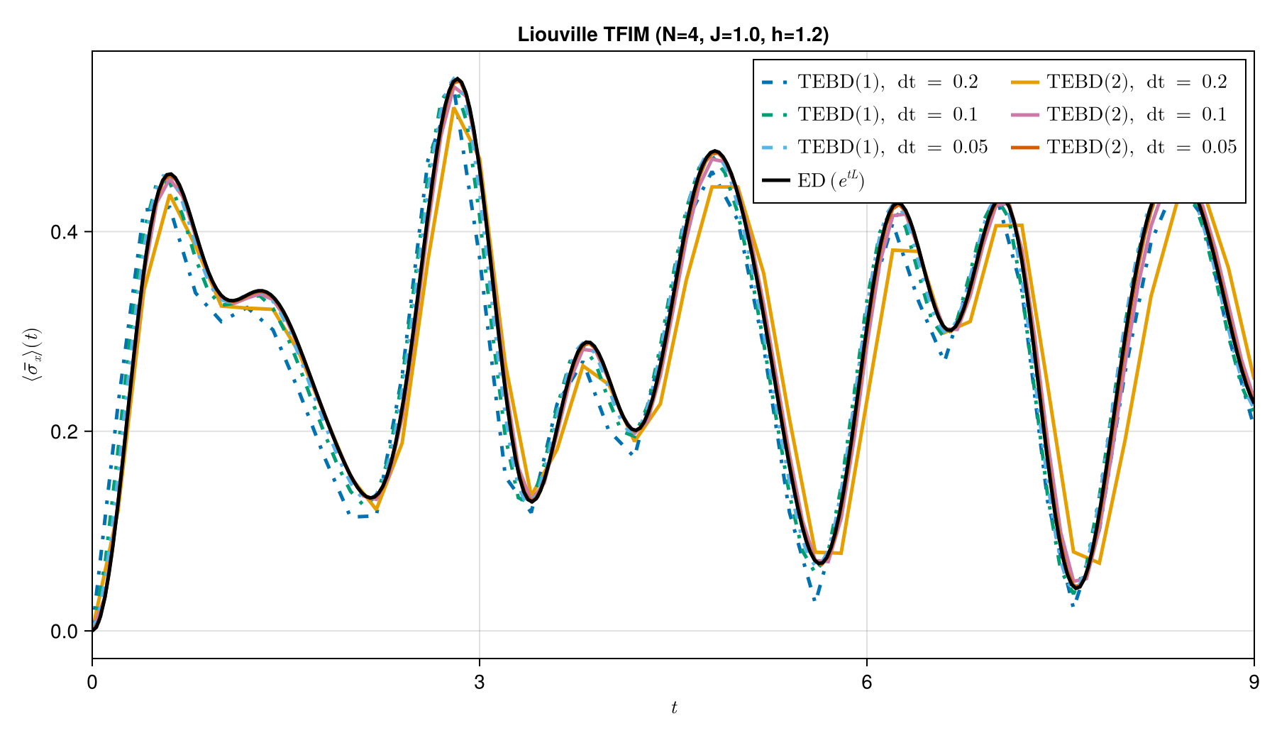
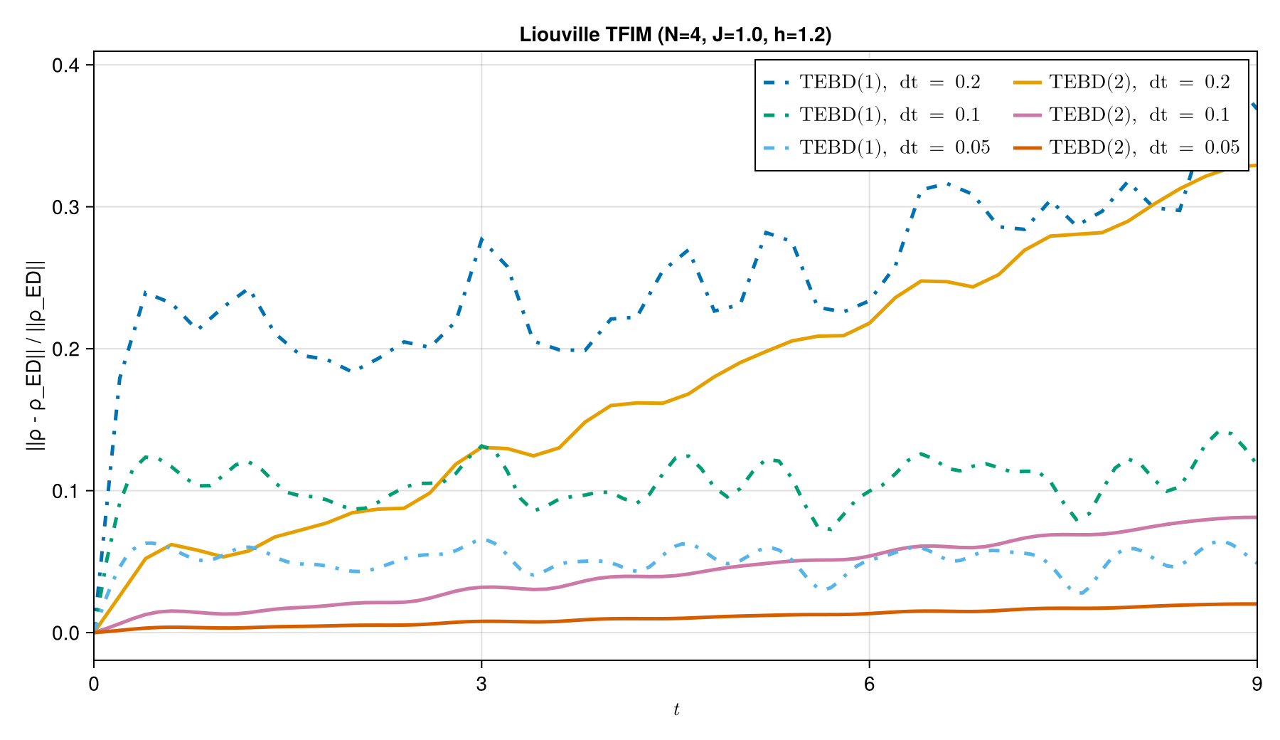
The Liouville trajectory is consistent with Hilbert TEBD. The final bond dimension is typically larger in Liouville space because one evolves a vectorized density matrix rather than a pure-state MPS.

The corresponding Liouville-space figures are: