Spin-bath process tensor

This example builds a process tensor for a spin coupled to a spin bath. We first use a single bath mode, then repeat the same idea with several bath modes.

The point of the example is not only to reproduce reduced dynamics. The point is to see the process tensor itself as the reusable object. Once the bath has been absorbed into this object, we can probe the system with different preparations, uninterrupted evolution, observable readouts, and later more general instruments.

The object we build

A usual reduced-dynamics calculation evolves the joint system-environment state,

\[\rho_{SE}(t) = U(t)\,\rho_S(0)\otimes\rho_E(0)\,U^\dagger(t),\]

and then traces out the environment,

\[\rho_S(t) = \operatorname{Tr}_E[\rho_{SE}(t)].\]

A process tensor reorganizes this computation. Instead of repeating the full system-environment evolution for every system-level question, we integrate out the environment once and store its influence as a tensor network in time.

Conceptually, a process tensor acts as a multi-time map,

\[\rho_S(t_n) = \mathcal{T}_{n:0} \left[ \mathcal{A}_{n-1},\ldots,\mathcal{A}_1,\rho_S(0) \right],\]

where the maps $\mathcal{A}_k$ are the interventions or instruments inserted on the system at intermediate times.

In this package, the process tensor is represented as a PT-MPO. Its memory bonds carry the bath influence between different time steps. Once this object is built, the bath no longer appears explicitly in the user-facing reduced calculation.

Physical model

We use one system spin with Hamiltonian

\[H_S = S_x.\]

The bath is made of one or more spin modes. A single mode has Hamiltonian

\[H_B = \omega S_x,\]

and couples to the system through

\[H_{SB} = g\,S_z^{(B)} S_z^{(S)}.\]

Both the system and bath modes start in the up state.

Setup

using Printf
using ProcessTensors
using ITensors
using LinearAlgebra
using ITensors.Ops: Exact, Trotter

const dt = 0.1
const nsteps = 24
const final_time = dt * nsteps
const joint_ed_frob_tol_single = 0.08
const joint_ed_frob_tol_multimode = 0.05
const dsys = 2
const denv_single = 2
const nmodes = 4
const denv_multimode = 2^nmodes
const mode_w = [0.5 + 0.1 * m for m in 1:nmodes]
const mode_g = [0.2 + 0.3 * m for m in 1:nmodes]

function print_pt_summary(label::AbstractString, result, frob_tol::Float64)
    @printf("%s\n", label)
    @printf("  max ‖ρ_PT − ρ_joint ED‖_F = %.3e\n", result.max_frob)
    @printf("  ⟨σ_x⟩ at t=0 (PT / ED)     = %.6f / %.6f\n", result.sx_pt[1], result.sx_ed[1])
    @printf("  ⟨σ_x⟩ at t=T (PT / ED)     = %.6f / %.6f\n", result.sx_pt[end], result.sx_ed[end])
    println()
    @assert all(isfinite, result.sx_pt) && all(isfinite, result.sx_ed)
    @assert all(isfinite, result.frob_err)
    @assert result.max_frob < frob_tol
end

print_pt_summary (generic function with 1 method)

Exact diagonalization reference

To audit the process-tensor construction on this small system, we compare the reduced states from evolve against exact joint Liouville evolution of the combined system and bath,

\[|\rho_{SE}(t)\rangle\rangle = e^{t\mathcal{L}_{SE}}|\rho_{SE}(0)\rangle\rangle,\]

followed by a partial trace over the bath Hilbert space,

\[\rho_S(t) = \operatorname{Tr}_E[\rho_{SE}(t)].\]

The helpers below convert Liouville MPS/MPO objects to dense matrices, extract the reduced system state, and report Frobenius errors along the trajectory. They are used only for this validation block.

σx = ComplexF64[0 1; 1 0]
σy = ComplexF64[0 -im; im 0]
σz = ComplexF64[1 0; 0 -1]

function pauli_expectations(ρ::AbstractMatrix{<:Number})
    return real(tr(ρ * σx)), real(tr(ρ * σy)), real(tr(ρ * σz))
end

function reduced_system_ρ(state_l, dsys::Int)
    rho_h = to_hilbert(state_l)
    sites = [
        only(filter(i -> plev(i) == 0 && hastags(i, "Site"), inds(rho_h.core[j])))
        for j in eachindex(rho_h.core)
    ]
    T = foldl(*, rho_h)
    A = Array(T, prime.(sites)..., sites...)
    return reshape(ComplexF64.(A), dsys, dsys)
end

function partial_trace_system(rho_h, dsys::Int, denv::Int)
    sites = [
        only(filter(i -> plev(i) == 0 && hastags(i, "Site"), inds(rho_h.core[j])))
        for j in eachindex(rho_h.core)
    ]
    T = foldl(*, rho_h)
    A = Array(T, prime.(sites)..., sites...)
    ρ4 = reshape(ComplexF64.(A), dsys, denv, dsys, denv)
    ρ_red = zeros(ComplexF64, dsys, dsys)
    for e in 1:denv
        ρ_red .+= @view ρ4[:, e, :, e]
    end
    return ρ_red
end

function compare_trajectory_to_joint_ed(trajectory, rho_sys0_h, system, H_full, joint_liouv, rho_joint0_l, denv::Int)
    sx_pt, sx_ed = Float64[], Float64[]
    frob_err = Float64[]

    ρ_pt = reduced_system_ρ(to_liouville(rho_sys0_h; sites=system.sites), dsys)
    ρ_ed = partial_trace_system(to_hilbert(rho_joint0_l), dsys, denv)
    push!(sx_pt, pauli_expectations(ρ_pt)[1])
    push!(sx_ed, pauli_expectations(ρ_ed)[1])
    push!(frob_err, norm(ρ_pt - ρ_ed))

    for k in 1:nsteps
        t = k * dt
        ρ_pt = reduced_system_ρ(trajectory.states_liouville[k], dsys)
        U_L = liouvillian_propagator(H_full, joint_liouv, t; alg=Exact())
        rho_joint_l = apply(U_L, copy(rho_joint0_l); cutoff=0.0, maxdim=typemax(Int))
        ρ_ed = partial_trace_system(to_hilbert(rho_joint_l), dsys, denv)
        push!(sx_pt, pauli_expectations(ρ_pt)[1])
        push!(sx_ed, pauli_expectations(ρ_ed)[1])
        push!(frob_err, norm(ρ_pt - ρ_ed))
    end

    return (; sx_pt, sx_ed, frob_err, max_frob=maximum(frob_err))
end

compare_trajectory_to_joint_ed (generic function with 1 method)

Single-mode spin bath

We first couple one system spin to one bath spin.

sys_phys = siteinds("S=1/2", 1)
env_phys = siteinds("S=1/2", 1)
env_liouv = liouv_sites(env_phys)

H_sys = OpSum()
H_sys += 1.0, "Sx", 1
system = spin_system(sys_phys, H_sys)

ρ_env0_h = to_dm(MPS(env_phys, ["Up"]))
ρ_env0_l = to_liouville(ρ_env0_h; sites=env_liouv)

H_env = OpSum()
H_env += 1.0, "Sx", 1

coupling = OpSum()
coupling += 1.0, "Sz", 1, "Sz", 2

mode = spin_mode(env_liouv, H_env, ρ_env0_l; coupling=coupling)
bath = spin_bath([mode])

ProcessTensors.SpinBath
  modes: 1
  space: Liouville
  site dims: 4
  bath Liouville dimension: 4

  mode summary:
    [1] SpinMode(dim=4, H_terms=1, coupling_terms=1)

Build the process tensor

The bath is integrated out here. The returned ProcessTensor stores the environment influence on the system across all time steps.

sys_alg=Trotter{2}() uses the second-order timestep sandwich $M(Δt/2)·Q·M(Δt/2)$ of free-system maps around each bath core (smaller time-discretization error than the default asymmetric Trotter{1}() layout).

pt_single = build_process_tensor(
    system,
    system.sites[1];
    environment=bath,
    dt=dt,
    nsteps=nsteps,
    alg=Exact(),
    sys_alg=Trotter{2}(),
)

println("Single-mode process tensor:")
println(pt_single)

@assert pt_single isa ProcessTensor
@assert pt_single.nsteps == nsteps
@assert pt_single.dt == dt

Single-mode process tensor:
24-step ProcessTensor{SpinSystem, SpinBath} | dt=0.1 | t_final=2.4 | maxlinkdim=4

  system:      SpinSystem(nsites=1, dissipative=false)
  environment: SpinBath(nmodes=1, D_bath=4, coupling=true)
  core:        MPO{Liouville}(length=24, linkdims=[4, 4, 4, …, 4])

Probe with instruments

Once pt_single exists, reduced questions are asked by contracting it with an instrument schedule.

evolve(pt, ρ0) is the convenience interface for uninterrupted evolution: prepare the initial state, let the system pass through each time step, and read out the reduced states at the requested times.

evaluate_process(pt, seq) exposes the same contraction with an explicit InstrumentSeq. Bind ObservableMeasurement to the PT output leg at the final time label (output_sites(pt, pt.nsteps - 1)) so the instrument ITensor contracts with the reduced state without index warnings.

ρ_sys0_h = to_dm(MPS(sys_phys, ["Up"]))

trajectory_single = evolve(pt_single, ρ_sys0_h)
println("evolve returned $(length(trajectory_single.times)) snapshots")

Sz = OpSum()
Sz += 1.0, "Sz", 1
k_final = pt_single.nsteps - 1
final_sites = output_sites(pt_single, k_final)

seq_final_sz = default_schedule(pt_single)
add!(seq_final_sz, state_preparation(ρ_sys0_h), 0)
add!(seq_final_sz, observable_measurement(Sz, final_sites), pt_single.nsteps)
final_sz_schedule = evaluate_process(pt_single, seq_final_sz)

Sz_obs = ProcessTensors.Instruments.instrument_itensor(
    observable_measurement(Sz, final_sites),
    final_sites,
    k_final,
)
ρ_final_T = foldl(*, trajectory_single.states_liouville[end])
final_sz_evolve = real(inner(ρ_final_T, Sz_obs))

println("Final ⟨σ_z⟩ from evaluate_process: ", real(final_sz_schedule))
println("Final ⟨σ_z⟩ from evolve:           ", final_sz_evolve)
@assert abs(real(final_sz_schedule) - final_sz_evolve) < 1e-8

evolve returned 24 snapshots
Final ⟨σ_z⟩ from evaluate_process: -0.2815676794556782
Final ⟨σ_z⟩ from evolve:           -0.2815676794556782

Validate against joint ED

joint_phys = Index[sys_phys[1], env_phys[1]]
joint_liouv_single = liouv_sites(joint_phys)

H_full_single = OpSum()
H_full_single += 1.0, "Sx", 1
H_full_single += 1.0, "Sx", 2
H_full_single += 1.0, "Sz", 1, "Sz", 2

psi_joint = MPS(joint_phys, ["Up", "Up"])
ρ_joint0_l_single = to_liouville(to_dm(psi_joint); sites=joint_liouv_single)

result_single = compare_trajectory_to_joint_ed(
    trajectory_single,
    ρ_sys0_h,
    system,
    H_full_single,
    joint_liouv_single,
    ρ_joint0_l_single,
    denv_single,
)
print_pt_summary("Single-mode spin bath", result_single, joint_ed_frob_tol_single)
println("Final ⟨σ_x⟩ (PT): ", result_single.sx_pt[end])

Single-mode spin bath
  max ‖ρ_PT − ρ_joint ED‖_F = 2.466e-04
  ⟨σ_x⟩ at t=0 (PT / ED)     = 0.000000 / 0.000000
  ⟨σ_x⟩ at t=T (PT / ED)     = 0.090204 / 0.090215

Final ⟨σ_x⟩ (PT): 0.09020417984812482

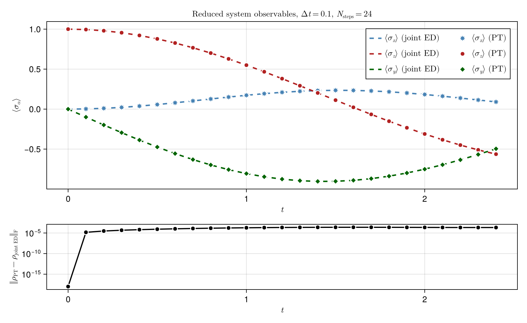
The plotting script compares all Pauli expectations and shows the Frobenius error on a log scale in the lower panel.

Multimode spin bath

The multimode case changes the bath, not the process-tensor idea. We couple the same system spin to several independent bath spins,

\[H_B^{(m)} = \omega_m S_x^{(m)}, \qquad H_{SB}^{(m)} = g_m S_z^{(m)} S_z^{(S)}.\]

env_phys_multi = siteinds("S=1/2", nmodes)
env_liouv_multi = liouv_sites(env_phys_multi)

modes = SpinMode[]
for m in 1:nmodes
    ρ_env_h = to_dm(MPS([env_phys_multi[m]], ["Up"]))
    ρ_env_l = to_liouville(ρ_env_h; sites=[env_liouv_multi[m]])

    H_mode = OpSum()
    H_mode += mode_w[m], "Sx", 1

    coupling_m = OpSum()
    coupling_m += mode_g[m], "Sz", 1, "Sz", 2

    push!(modes, spin_mode([env_liouv_multi[m]], H_mode, ρ_env_l; coupling=coupling_m))
end
bath_multi = spin_bath(modes)

ProcessTensors.SpinBath
  modes: 4
  space: Liouville
  site dims: 4, 4, 4, 4
  bath Liouville dimension: 256

  mode summary:
    [1] SpinMode(dim=4, H_terms=1, coupling_terms=1)
    [2] SpinMode(dim=4, H_terms=1, coupling_terms=1)
    [3] SpinMode(dim=4, H_terms=1, coupling_terms=1)
    [4] SpinMode(dim=4, H_terms=1, coupling_terms=1)

Build the process tensor

pt_multi = build_process_tensor(
    system,
    system.sites[1];
    environment=bath_multi,
    dt=dt,
    nsteps=nsteps,
    alg=Exact(),
    sys_alg=Trotter{2}(),
)

println("Multimode process tensor ($nmodes bath spins):")
println(pt_multi)

@assert pt_multi isa ProcessTensor
@assert maxlinkdim(pt_multi) >= maxlinkdim(pt_single)

Multimode process tensor (4 bath spins):
24-step ProcessTensor{SpinSystem, SpinBath} | dt=0.1 | t_final=2.4 | maxlinkdim=256

  system:      SpinSystem(nsites=1, dissipative=false)
  environment: SpinBath(nmodes=4, D_bath=256, coupling=true)
  core:        MPO{Liouville}(length=24, linkdims=[256, 256, 256, …, 256])

Probe with instruments

trajectory_multi = evolve(pt_multi, ρ_sys0_h)
println("evolve returned $(length(trajectory_multi.times)) snapshots")

final_sites_multi = output_sites(pt_multi, pt_multi.nsteps - 1)
seq_multi_sz = default_schedule(pt_multi)
add!(seq_multi_sz, state_preparation(ρ_sys0_h), 0)
add!(seq_multi_sz, observable_measurement(Sz, final_sites_multi), pt_multi.nsteps)
final_sz_multi = evaluate_process(pt_multi, seq_multi_sz)

Sz_obs_multi = ProcessTensors.Instruments.instrument_itensor(
    observable_measurement(Sz, final_sites_multi),
    final_sites_multi,
    pt_multi.nsteps - 1,
)
ρ_final_multi_T = foldl(*, trajectory_multi.states_liouville[end])
final_sz_multi_evolve = real(inner(ρ_final_multi_T, Sz_obs_multi))

println("Final ⟨σ_z⟩ from evaluate_process: ", real(final_sz_multi))
println("Final ⟨σ_z⟩ from evolve:           ", final_sz_multi_evolve)
@assert abs(real(final_sz_multi) - final_sz_multi_evolve) < 1e-8

evolve returned 24 snapshots
Final ⟨σ_z⟩ from evaluate_process: 0.07629696177989548
Final ⟨σ_z⟩ from evolve:           0.07629696177989548

Validate against joint ED

joint_phys_multi = Index[sys_phys[1], env_phys_multi...]
joint_liouv_multi = liouv_sites(joint_phys_multi)

H_full_multi = let
    H = OpSum()
    H += 1.0, "Sx", 1
    for m in 1:nmodes
        H += mode_w[m], "Sx", m + 1
        H += mode_g[m], "Sz", m + 1, "Sz", 1
    end
    H
end

joint_init = vcat(["Up"], fill("Up", nmodes))
psi_joint_multi = MPS(joint_phys_multi, joint_init)
ρ_joint0_l_multi = to_liouville(to_dm(psi_joint_multi); sites=joint_liouv_multi)

result_multi = compare_trajectory_to_joint_ed(
    trajectory_multi,
    ρ_sys0_h,
    system,
    H_full_multi,
    joint_liouv_multi,
    ρ_joint0_l_multi,
    denv_multimode,
)
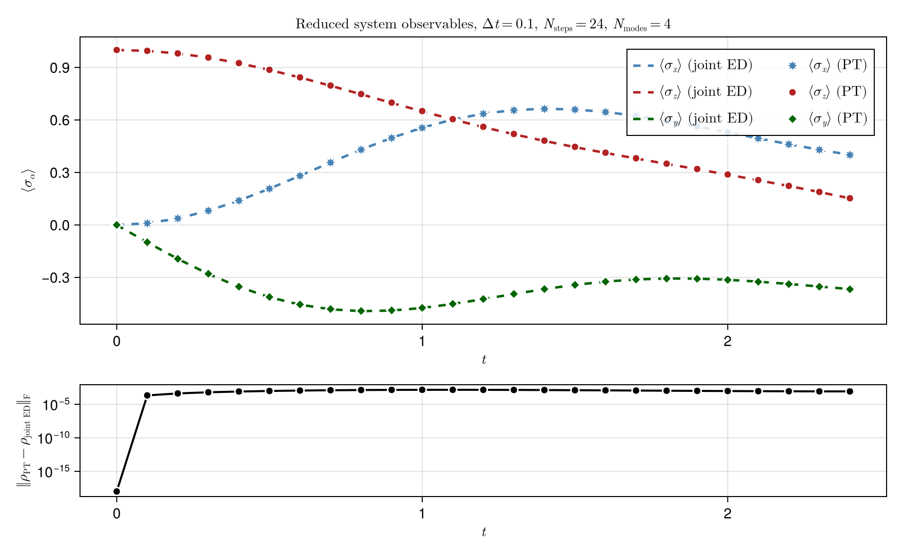
print_pt_summary("Multimode spin bath ($nmodes modes)", result_multi, joint_ed_frob_tol_multimode)
println("Final ⟨σ_x⟩ (PT): ", result_multi.sx_pt[end])

Multimode spin bath (4 modes)
  max ‖ρ_PT − ρ_joint ED‖_F = 1.453e-03
  ⟨σ_x⟩ at t=0 (PT / ED)     = 0.000000 / 0.000000
  ⟨σ_x⟩ at t=T (PT / ED)     = 0.400195 / 0.400626

Final ⟨σ_x⟩ (PT): 0.40019494558570495

What controls the error?

The main algorithmic error comes from the short-time system–bath split inside build_process_tensor. Prefer sys_alg=Trotter{2}() (second-order sandwich) over the default Trotter{1}() asymmetric layout when time-discretization error dominates; smaller dt further reduces that residual. In larger calculations, also monitor PT-MPO bond truncation (cutoff, maxdim) and accumulated roundoff in long contractions.

Here is a direct comparison at fixed $Δt$ up to $t = 1.5$. We build two single-mode process tensors that differ only in sys_alg, ask evaluate_process for the final $⟨S^x⟩$ (ITensor S=1/2 spin operator), and compare both answers to joint continuous-time ED.

T_cmp = 1.5
nsteps_cmp = round(Int, T_cmp / dt)
@assert isapprox(nsteps_cmp * dt, T_cmp; atol=1e-12)

pt_order1 = build_process_tensor(
    system,
    system.sites[1];
    environment=bath,
    dt=dt,
    nsteps=nsteps_cmp,
    alg=Exact(),
    sys_alg=Trotter{1}(),
)
pt_order2 = build_process_tensor(
    system,
    system.sites[1];
    environment=bath,
    dt=dt,
    nsteps=nsteps_cmp,
    alg=Exact(),
    sys_alg=Trotter{2}(),
)

Sx = OpSum()
Sx += 1.0, "Sx", 1

function final_sx_evaluate(pt)
    out = output_sites(pt, pt.nsteps - 1)
    seq = default_schedule(pt)
    add!(seq, state_preparation(ρ_sys0_h), 0)
    add!(seq, observable_measurement(Sx, out), pt.nsteps)
    return real(evaluate_process(pt, seq))
end

sx_t1 = final_sx_evaluate(pt_order1)
sx_t2 = final_sx_evaluate(pt_order2)

U_ed = liouvillian_propagator(H_full_single, joint_liouv_single, T_cmp; alg=Exact())
ρ_joint_ed = apply(U_ed, copy(ρ_joint0_l_single); cutoff=0.0, maxdim=typemax(Int))
ρ_ed = partial_trace_system(to_hilbert(ρ_joint_ed), dsys, denv_single)

sx_ed = real(tr(ρ_ed * (σx / 2)))

err_t1 = abs(sx_t1 - sx_ed)
err_t2 = abs(sx_t2 - sx_ed)

@printf("⟨Sˣ⟩(t=%.1f)  Trotter{1} / Trotter{2} / ED = %.6f / %.6f / %.6f\n", T_cmp, sx_t1, sx_t2, sx_ed)
@printf("|⟨Sˣ⟩_PT − ⟨Sˣ⟩_ED|  Trotter{1} = %.3e,  Trotter{2} = %.3e\n", err_t1, err_t2)
@assert err_t2 < err_t1
@assert err_t2 < 0.1 * err_t1

⟨Sˣ⟩(t=1.5)  Trotter{1} / Trotter{2} / ED = 0.108877 / 0.117688 / 0.117576
|⟨Sˣ⟩_PT − ⟨Sˣ⟩_ED|  Trotter{1} = 8.698e-03,  Trotter{2} = 1.125e-04