Multi-time correlations

A process tensor stores how an environment carries information between different intervention times. Once it is built, changing the instruments on its time legs gives different multi-time observables without rebuilding the system–environment dynamics.

Here we evaluate

\[C_{zz}(t_2,t_1) = \langle \sigma_z(t_2)\sigma_z(t_1)\rangle\]

for a system spin coupled to one bath spin.

Spin-bath process tensor

We use

\[H_S=S_x,\qquad H_E=S_x,\qquad H_{SE}=S_z\otimes S_z,\]

with the system initially in $|\mathrm{Dn}\rangle$ and the bath in $|\mathrm{Up}\rangle$.

using ITensors
using LinearAlgebra: diag
using ProcessTensors

const dt = 0.5
const n_times = 6
const pt_nsteps = n_times + 1

system_sites = siteinds("S=1/2", 1)
bath_sites = siteinds("S=1/2", 1)
bath_liouville_sites = liouv_sites(bath_sites)

H_system = OpSum()
H_system += 1.0, "Sx", 1
system = spin_system(system_sites, H_system)

H_bath = OpSum()
H_bath += 1.0, "Sx", 1

H_coupling = OpSum()
H_coupling += 1.0, "Sz", 1, "Sz", 2

bath_state = to_dm(MPS(bath_sites, ["Up"]))
bath_state_liouville =
    to_liouville(bath_state; sites=bath_liouville_sites)

bath_mode = spin_mode(
    bath_liouville_sites,
    H_bath,
    bath_state_liouville;
    coupling=H_coupling,
)
bath = spin_bath([bath_mode])

process_tensor = build_process_tensor(
    system,
    system.sites[1];
    environment=bath,
    dt=dt,
    nsteps=pt_nsteps,
)

@assert process_tensor.nsteps == pt_nsteps
@assert process_tensor.dt == dt

Two-time instrument schedules

A two-time correlator is not computed by first producing a reduced trajectory and then multiplying numbers. The operator insertions are part of the process.

For t₂ > t₁, the two-time correlation of A and B is given as

\[\begin{aligned} \langle A(t_2) B(t_1) \rangle &= \operatorname{Tr}[U^{\dagger}(t_2) A\, U(t_2-t_1)\, B\, U(t_1)\, \rho(0)] \\ &= \operatorname{Tr}[U^{\dagger}(t_2-t_1) A\, U(t_2-t_1)\, B\, \rho(t_1)] \\ &= \operatorname{Tr}\left[A\, U(t_2-t_1)\, B\, \rho(t_1)\, U^{\dagger}(t_2-t_1)\right] \\ &= \operatorname{Tr}\left[A\, U(t_2-t_1)\, \rho_{B_L}(t_1)\, U^{\dagger}(t_2-t_1)\right] \\ &= \operatorname{Tr}\left[A\, \rho_{B_L}(t_2)\right]. \end{aligned}\]

In simple words, we evolve $\rho(0)$ forward to $t_1$, aply B from the left, evolve the resultant object to $t_2$, and measure the expectation of $A$. This can be implemented as the following instrument sequence:

t = 0      : state_preparation(ρ₀)
t = t₁    : insert B from the left
t = t₂    : insert A
after t₂  : propagate with identity operations and TraceOut

For t₁ > t₂, the earlier operator and the later operator exchange roles. The implementation must also keep track of whether the early insertion acts from the left or from the right, so that the product ordering in ⟨A(t₂)B(t₁)⟩ is represented correctly.

On the diagonal t₂ = t₁, both operators are inserted at the same time. The same-time instrument represents the product at that single time leg.

The package helper two_time_correlation_seq builds this InstrumentSeq for us, considering all the above cases. Then evaluate_process contracts the process tensor with that sequence.

system_state = to_dm(MPS(system_sites, ["Dn"]))

sigma_z = OpSum()
sigma_z += 2.0, "Sz", 1

sequence = two_time_correlation_seq(
    process_tensor,
    (sigma_z, 2),
    (sigma_z, 1);
    rho0=system_state,
)

correlation = evaluate_process(process_tensor, sequence)

@assert correlation isa ComplexF64
@assert isfinite(correlation)

Correlation grid

Each grid entry differs only by the two insertion times. The same process tensor is reused throughout:

time_indices = 0:(n_times - 1)
times = dt .* collect(time_indices)

Czz = [
    evaluate_process(
        process_tensor,
        two_time_correlation_seq(
            process_tensor,
            (sigma_z, t2),
            (sigma_z, t1);
            rho0=system_state,
        ),
    )
    for t1 in time_indices, t2 in time_indices
]

diagonal_error = maximum(abs.(diag(Czz) .- 1))
conjugate_error = maximum(abs.(Czz - Czz'))

@assert all(isfinite, Czz)
@assert diagonal_error < 1e-10
@assert conjugate_error < 1e-10

You can run the dedicated script to evaluate the three correlator grids to produce the following heatmaps:

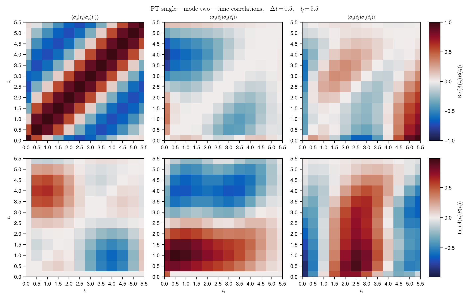
The first panel is an autocorrelation:

\[C_{zz}(t_2,t_1) = \langle \sigma_z(t_2)\sigma_z(t_1)\rangle .\]

Since σz is Hermitian and σz² = I, the diagonal is a sanity check:

\[C_{zz}(t,t) = 1 .\]

Therefore the real diagonal should be close to one, and the imaginary diagonal should be close to zero. Off the diagonal, the autocorrelation satisfies the conjugate structure

\[C_{zz}(t_2,t_1)^* = C_{zz}(t_1,t_2),\]

so the real part is symmetric while the imaginary part is antisymmetric.

For cross-correlations, the structure is different. For example,

\[\sigma_z\sigma_x = i\sigma_y,\qquad \sigma_x\sigma_y = i\sigma_z .\]

Thus the equal-time diagonal of ⟨σz(t₂)σx(t₁)⟩ is expected to be mainly imaginary and related to ⟨σy(t)⟩, while the equal-time diagonal of ⟨σx(t₂)σy(t₁)⟩ is related to ⟨σz(t)⟩. Away from the diagonal, there is no reason for a single cross-correlation grid to be symmetric; the conjugate partner involves the reversed operator ordering.