Dissipative spin-chain dynamics

A closed transverse-field Ising model describes coherent spin rotation and correlated many-body motion. Real spin platforms also exchange energy with their surroundings, so coherent dynamics is progressively damped and the system relaxes toward a state selected by both the Hamiltonian and the environment.

Adding local amplitude damping gives a standard open-system benchmark. The dissipative transverse-field Ising chain is a paradigmatic model of correlated open-system dynamics, widely used to study relaxation, decoherence, and nonequilibrium steady states. Here it also provides a compact example of the ProcessTensors.jl workflow:

1. define a physical Hamiltonian as an OpSum;
2. specify local Lindblad channels as jump_ops;
3. vectorize the initial density matrix;
4. evolve it directly with Liouville-space tebd.

Model and physical scales

We use an open transverse-field Ising chain,

\[H = -J\sum_{j=1}^{N-1} Z_jZ_{j+1} -h\sum_{j=1}^{N} X_j ,\]

together with a local loss channel at each site,

\[L_j=S_j^-, \qquad j=1,\ldots,N,\]

so the density matrix evolves as

\[\frac{d\rho}{dt} = -i[H,\rho] + \gamma\sum_{j=1}^{N}\mathcal{D}[S_j^-]\rho , \qquad \mathcal{D}[L]\rho = L\rho L^\dagger -\frac{1}{2}\{L^\dagger L,\rho\}.\]

The Ising term correlates neighboring spins, the transverse field rotates them away from the $Z$ axis, and $S_j^-$ transfers local Up population to Dn. The rates $J$, $h$, and $\gamma$ therefore set competing coherent, interaction, and relaxation timescales.

We start from the fully polarized state $|\mathrm{Up}\cdots\mathrm{Up}\rangle$ and monitor two complementary observables:

\[\bar n_\uparrow(t) = \frac{1}{N}\sum_{j=1}^{N} \left\langle\frac{I+Z_j}{2}\right\rangle_t , \qquad \overline X(t) = \frac{1}{N}\sum_{j=1}^{N}\langle X_j\rangle_t .\]

The excited-spin density $\bar n_\uparrow$ tracks population relaxation under amplitude damping. The transverse magnetization $\overline X$ exposes the coherent response generated by the transverse field.

Parameters and operators

using Printf
using ITensors
using ITensors.Ops: Trotter
using ProcessTensors

const N = 6
const J = 1.0
const transverse_field = 1.2
const decay_rate = 0.5
const dt = 0.1
const final_time = 4.0
const maxdim = 96
const cutoff = 1e-10

physical_sites = siteinds("S=1/2", N)
liouville_sites = liouv_sites(physical_sites)

hamiltonian = let H = OpSum()
    for j in 1:(N - 1)
        H += -J, "Z", j, "Z", j + 1
    end
    for j in 1:N
        H += -transverse_field, "X", j
    end
    H
end

sum(
  -1.0 Z(1,) Z(2,)
  -1.0 Z(2,) Z(3,)
  -1.0 Z(3,) Z(4,)
  -1.0 Z(4,) Z(5,)
  -1.0 Z(5,) Z(6,)
  -1.2 X(1,)
  -1.2 X(2,)
  -1.2 X(3,)
  -1.2 X(4,)
  -1.2 X(5,)
  -1.2 X(6,)
)

A tuple (γ, "S-", j) contributes $\gamma\mathcal D[S_j^-]$ to the Liouvillian. The first entry is the dissipative rate, the second entry is the jump operator responsible for the dissipation, and the third is the site index where this operator sits.

jump_operators = [(decay_rate, "S-", j) for j in 1:N]

initial_state = MPS(physical_sites, fill("Up", N))
initial_density = to_dm(initial_state)
initial_density_liouville =
    to_liouville(initial_density; sites=liouville_sites)

mean_x_operator = let observable = OpSum()
    for j in 1:N
        observable += 1 / N, "X", j
    end
    observable
end

sum(
  0.16666666666666666 X(1,)
  0.16666666666666666 X(2,)
  0.16666666666666666 X(3,)
  0.16666666666666666 X(4,)
  0.16666666666666666 X(5,)
  0.16666666666666666 X(6,)
)

Now we define the observables we wish to track in the Liouville space. Local projector onto Up is $(I + Z)/2$, and the local transverse magnetization is $X/N$.

excited_density_operator = let observable = OpSum()
    for j in 1:N
        observable += 0.5 / N, "Id", j
        observable += 0.5 / N, "Z", j
    end
    observable
end

mean_x_liouville = to_liouville(
    MPO(mean_x_operator, physical_sites);
    sites=liouville_sites,
)
excited_density_liouville = to_liouville(
    MPO(excited_density_operator, physical_sites);
    sites=liouville_sites,
)

@assert isapprox(real(tr(initial_density)), 1.0; atol=1e-12)

Liouville-space TEBD

Vectorization turns the master equation into

\[\frac{d}{dt}|\rho(t)\rangle\rangle = \mathcal L|\rho(t)\rangle\rangle .\]

tebd constructs local Liouville-space gates internally from the physical Hamiltonian and the jump tuples. A second-order Suzuki–Trotter decomposition approximates $e^{\mathcal L\Delta t}$; because the generator already contains the Hamiltonian factor $-i$, the evolution time passed to Liouville TEBD is the real interval dt.

nsteps = round(Int, final_time / dt)
@assert isapprox(nsteps * dt, final_time; atol=100eps(Float64))
times = collect(range(0.0; step=dt, length=nsteps + 1))

trajectory = let
    density = copy(initial_density_liouville)
    mean_x = Float64[]
    excited_density = Float64[]
    trace_errors = Float64[]
    bond_dimensions = Int[]

    for step in eachindex(times)
        trace_value = tr(to_hilbert(density))
        push!(mean_x, real(inner(mean_x_liouville, density) / trace_value))
        push!(
            excited_density,
            real(inner(excited_density_liouville, density) / trace_value),
        )
        push!(trace_errors, abs(trace_value - 1))
        push!(bond_dimensions, maxlinkdim(density))

        step == length(times) && continue

        density = tebd(
            density,
            hamiltonian,
            dt,
            dt;
            jump_ops=jump_operators,
            alg=Trotter{2}(),
            maxdim=maxdim,
            cutoff=cutoff,
            progress=false,
        )
    end

    (
        mean_x=mean_x,
        excited_density=excited_density,
        trace_errors=trace_errors,
        bond_dimensions=bond_dimensions,
    )
end

max_trace_error = maximum(trajectory.trace_errors)
max_bond_dimension = maximum(trajectory.bond_dimensions)

@assert all(isfinite, trajectory.mean_x)
@assert all(isfinite, trajectory.excited_density)
@assert all(value -> -1 - 1e-8 ≤ value ≤ 1 + 1e-8, trajectory.mean_x)
@assert all(value -> -1e-8 ≤ value ≤ 1 + 1e-8, trajectory.excited_density)
@assert max_trace_error < 1e-2

println("Dissipative transverse-field Ising chain")
@printf("  N=%d, J=%.2f, h=%.2f, γ=%.2f\n", N, J, transverse_field, decay_rate)
@printf(
    "  final ⟨X̄⟩ = %.6f, final n̄_↑ = %.6f\n",
    trajectory.mean_x[end],
    trajectory.excited_density[end],
)
@printf("  max trace error = %.3e, max bond dim = %d\n", max_trace_error, max_bond_dimension)

Dissipative transverse-field Ising chain
  N=6, J=1.00, h=1.20, γ=0.50
  final ⟨X̄⟩ = 0.157441, final n̄_↑ = 0.423257
  max trace error = 1.109e-03, max bond dim = 64

Relaxation and numerical interpretation

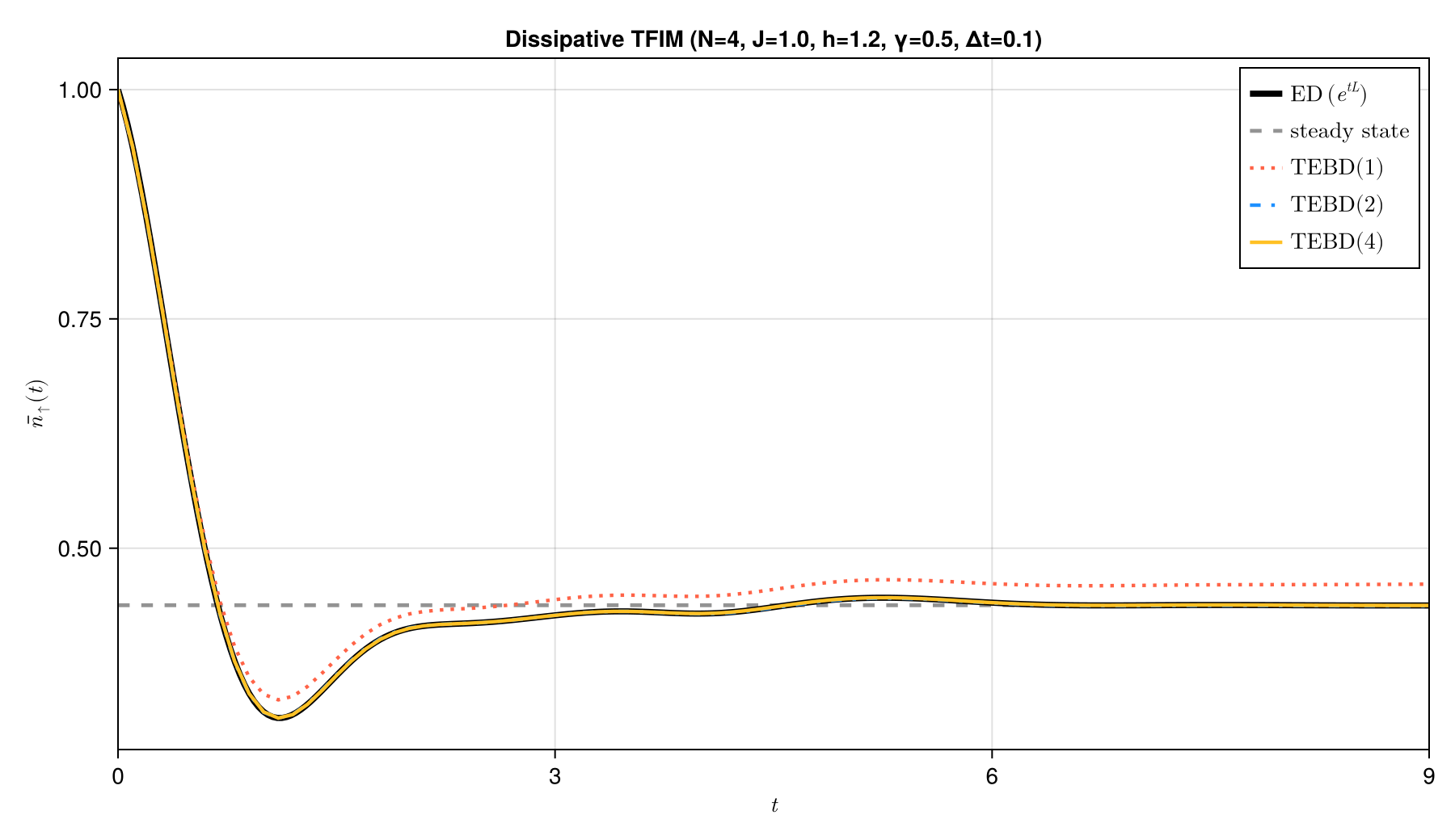
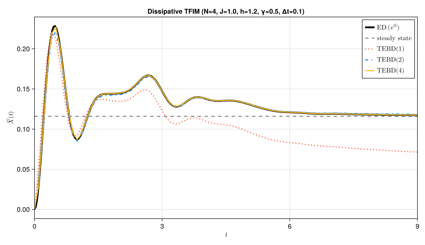
The initial all-Up state has unit excited-spin density. With time, local $S^-$ jump operators remove that population, thus $\bar n_\uparrow(t)$ falls toward a stationary value. The transverse field creates a non-zero coherent response, that leads to transient oscillations in the transverse magnetization. These oscillations are damped as the environment erases coherent spin motion by decaying the population, while the Ising coupling makes the response collective rather than a set of independent one-spin decays.

As a consequence, the late-time values are not ground-state observables of $H$. They describe a nonequilibrium stationary response determined by coherent rotation, spin–spin interactions, and local loss. The dense curves in the figures below validate that interpretation and show how the TEBD approximation improves as the Trotter order increases at fixed $\Delta t$.

Sources of numerical error

This calculation has three principal numerical approximations:

• Trotter error: local coherent and dissipative Liouvillian terms do not generally commute. At fixed $\Delta t$, raising the Suzuki–Trotter order from $1$ to $2$ to $4$ systematically reduces that splitting error.
• Tensor-network truncation: two-site gates can increase the Liouville-MPS bond dimension. cutoff and maxdim control the discarded information.
• Finite simulation window: final_time may be too short to establish that the stationary regime has been reached.

Trace drift is a useful inexpensive diagnostic, but it does not by itself prove positivity or convergence. The full script compares Trotter orders $1$, $2$, and $4$ at $\Delta t = 0.1$ with dense evolution on a smaller chain.